SPX x Markov
A review of regime switching models
Market regime detection and prediction is one of the most important realms of financial research. In this article, I review regime-switching models. I also implemented two models, Hamilton (1989) and KNS(1998), to mark SPX data spanning 100 years.
I am going to divide the article into three parts:
a) Markov Explainer
b) Switching Models
c) Switching models to date SPX
Markov explainer
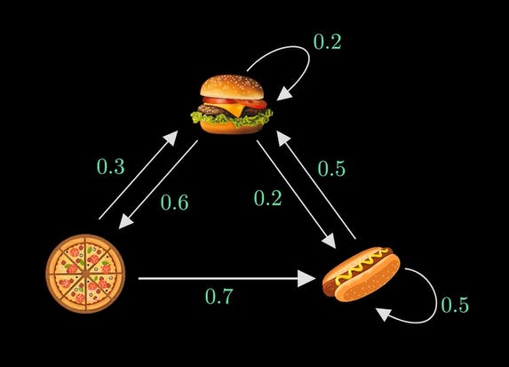
First off, let’s look at what a Markov chain is. Let’s say there’s a restaurant that serves only three items: Burger, Hotdog, and Pizza. But there’s a caveat; it only serves one kind of item on a particular day. Let’s say they are serving pizza today, now they have a choice of serving a burger or hotdog, and this choice is only dependent on what they are serving today and not on what they were serving in the previous days. This is what a Markov chain is all about.
These probabilities don’t change. This Markov chain doesn't care how you got there; it only cares about where you are right now. In the below image, the arrows are called the state transitions and the numbers on the arrows are the probabilities of those state transitions. It should be noted that the sum of the probabilities from a certain state should be equal to 1, as they are probabilities. By understanding these probabilities of transitions, we can make predictions and understand how things might change over time. The above example is taken from the Normalized Nerd Channel.
The following table is called the state transition matrix, which is basically the adjacency matrix of the graph (Markov chain).
Switching Models
Stock markets have a notion of states or regimes where they are in at a certain point of time. They are generally called the hot and cold periods. The switching models assume that the data generation process is governed by two different regimes (states) and estimate the unobserved states while allowing transition probabilities to follow a Markov chain. The results from these models can be used to date the previous time series or can also be helpful in forecasting the impending regimes. Usually, the sample is rolled forward by one observation, and the new set of model parameters and probability forecasts are estimated. Let’s say the model results say that the next period forecast that a certain asset is going to be in the low (cold) regime is more than 0.5, so we can make a decision to buy that asset or hold on to it.
Switching models to date SPX
For this article, I took the data of good old SPX from Kaggle, ranging from 30-12-1927 to 4-11-2020. I will be implementing two different switching models.
i) Hamilton (1989) Model
The model is an autoregressive model of order 4 in which the mean of the process switches between two regimes.
The matrix of transition probabilities:
We have to define the number of regimes using K_regimes argument and the order of the autoregression with order, the model is fit via MLE. It takes the log-likelihood function for the observed data, takes the derivative, and maximizes it to find the unknown parameters.
From these parameters, the transition probabilities can be calculated using the forward-backward algorithm. The forward pass calculates the (filtered) probabilities of being in a particular regime at each point, given all the observations until that point. The backward pass OTOH, calculates the (smoothed) probabilities of being in a particular regime at each point given all the observed data until the end of the time series.
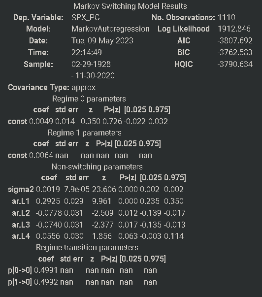
These were the results of the Hamilton model for our SPX data:
And here is a picture of the regime probabilities (both filtered and smoothed) throughout our time series:
ii) Kim, Nelson, and Startz (1998) Model
This model demonstrates estimation with regime heteroskedasticity (switching of variances) and no mean effect.
These were the results of the KNS model for our SPX data:
In this model, the whole time series is assumed to consist of 3 different states with low, high and medium variance.
Here is a picture of the regime probabilities throughout our time series in all 3 states:
From both of the model’s results we can see clear and nice markings of the regimes. Particularly the cold regimes of 1929 - 1933 (Great Depression), the Recession of 1937–1938, the Early 1990s recession, the 2007 crisis, and the recent early 2020 (COVID) are distinctly evident.
References:
Data source:
https://www.kaggle.com/datasets/henryhan117/sp-500-historical-data
Python Libraries:
https://www.statsmodels.org/dev/examples/notebooks/generated/markov_autoregression.html
YouTube Playlist explaining the Markov chain:
https://www.youtube.com/playlist?list=PLM8wYQRetTxBkdvBtz-gw8b9lcVkdXQKV
Cambridge University’s slides on Markov chain:
https://www.cambridge.org/my/download_file/193037/
List of Recessions:
https://en.wikipedia.org/wiki/List_of_recessions_in_the_United_States


